处理边缘
卷积边界问题及其处理
边界问题
 image
image
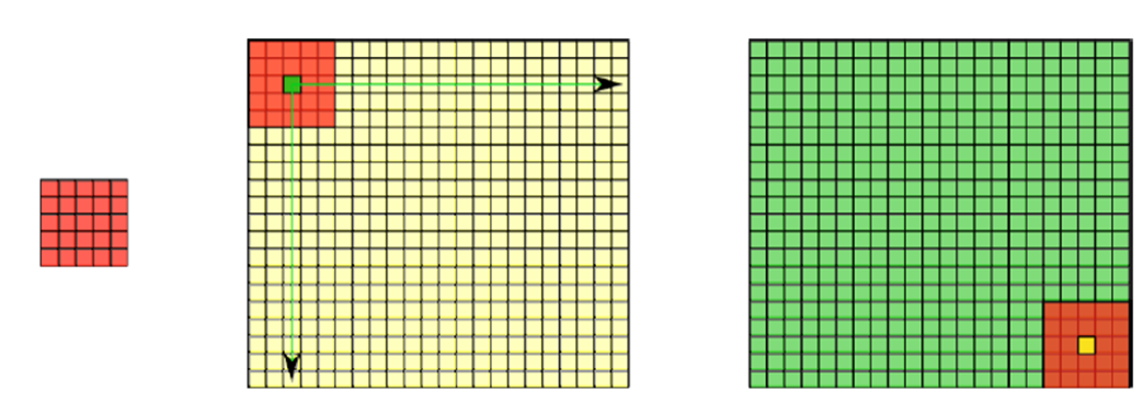
卷积边界问题是指的图像卷积的时候边界像素,不能被卷积操作,原因在于边界像素没有完全跟kernel重叠,所以当3x3滤波时候有1个像素(最上面一行的像素)的边缘没有被处理,5x5滤波的时候有2个像素的边缘没有被处理。
处理
在卷积开始之前增加边缘像素,填充的像素值为0或者RGB黑色,比如3x3在四周各填充1个像素的边缘,这样就确保图像的边缘被处理,在卷积处理之后再去掉这些边缘。openCV中默认的处理方法是: BORDER_DEFAULT,此外常用的还有如下几种:
- BORDER_CONSTANT:用指定像素填充边缘
- BORDER_REPLICATE:用已知边缘像素值来填充边缘像素值
- BORDER_WRAP:用另外一边的像素来补偿填充
下面是给图像自定义添加边缘
copyMakeBorder:给图像添加边缘API
copyMakeBorder(
  Mat src, // 输入图像
  Mat dst, // 添加边缘图像
  int top, // 边缘长度,一般上下左右都取相同值,
  int bottom,
  int left,
  int right,
  int borderType // 边缘类型
  Scalar value // Scalar用于指定颜色,边缘类型为 BORDER_CONSTANT 时,有效
)
下面代码展示一下如何具体使用:
int top = (int)0.05*src.rows;
int bottom = (int)0.05*src.rows;
int left = (int)0.05*src.cols;
int right = (int)0.05*src.cols;

Scalar color = Scalar(rng.uniform(0, 255), rng.uniform(0, 255), rng.uniform(0, 255));
copyMakeBorder(src, dst, top, bottom, left, right, borderType, color);
imshow(OUTPUT_WIN, dst);
这是完整演示四种方法如何切换的代码:
#include <opencv2/opencv.hpp>
#include <iostream>
#include <math.h>

using namespace cv;

Mat src, dst, kernal;

int main(int argc, char** argv) {
	src = imread("D:/1.jpg");
	if (!src.data) {
		printf("could not load image...\n");
		return -1;
	}

	char INPUT_WIN[] = "input image";
	char OUTPUT_WIN[] = "result image";
	namedWindow(INPUT_WIN, CV_WINDOW_AUTOSIZE);
	namedWindow(OUTPUT_WIN, CV_WINDOW_AUTOSIZE);
	imshow("input image", src);

	int top = 0.05*src.rows;
	int bottom = 0.05*src.rows;
	int left = 0.05*src.cols;
	int right = 0.05*src.cols;

	RNG rng(12345); //生成随机数
	int borderType = BORDER_DEFAULT;

	int c = 0;
	while (true)
	{
		c = waitKey(500);
		if ((char)c ==27 ) //按下键盘ESC对应的数值就是27,也就是按下键盘推出while循环
		{
			break;
		}
		if ((char)c == 'r')
		{
			borderType = BORDER_REPLICATE;
		}
		else if ((char)c == 'w')
		{
			borderType = BORDER_WRAP;
		}
		else if ((char)c == 'c')
		{
			borderType = BORDER_CONSTANT;
		}
		else if((char)c == 'd')
		{
			borderType = BORDER_DEFAULT;
		}
		Scalar color = Scalar(rng.uniform(0, 255), rng.uniform(0, 255), rng.uniform(0, 255)); //生成0-255之前随机颜色值
		copyMakeBorder(src, dst, top, bottom, left, right, borderType, color);
		imshow(OUTPUT_WIN, dst);
	}

	return 0;
}
Sobel算子
卷积的应用:图像边缘提取
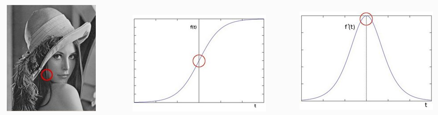
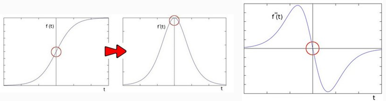
边缘是图像像素发生显著跃迁的地方,通过求一阶导数可以很好地捕捉边缘。
delta = f(x) – f(x-1), delta越大,说明像素在X方向变化越大,边缘信号越强。
 image
image
Sobel算子
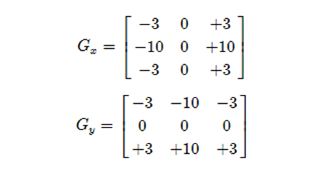
Sobel算子又被称为一阶微分算子,求导算子,在水平和垂直两个方向上求导,得到图像X方法与Y方向梯度图像。它是离散微分算子(discrete differentiation operator),用来计算灰度图像的近似梯度。
Soble算子功能集合高斯平滑和微分求导。
 image
image
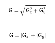
我们以水平梯度为例。他的水平方向上面变化十分的明显,在水平方向上给不同的权重,通过权重值来扩大差异。
 image
image
最终图像梯度如上图所示,一般为了让计算机算的更快一些,我们会取绝对值的形式。
Sobel算子API
cv::Sobel (
InputArray Src // 输入图像
OutputArray dst// 输出图像,大小与输入图像一致
int depth // 输出图像深度.
Int dx.  // X方向,几阶导数,如果想求x方向的时候就让这个数取1,y方向上取0
int dy // Y方向,几阶导数.
int ksize, SOBEL算子kernel大小,必须是1、3、5、7、
double scale  = 1
double delta = 0
int borderType = BORDER_DEFAULT
)
 image
image
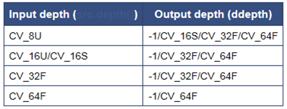
这里关于深度说一下,因为考虑两个图像像素之间的差值,可能做差之后超过255,超过255的8U灰度图像就会被截断,所以相比于输入,输出会上升一个层次。(-1就是表示选择和原先的一样)
Sobel算子改进版:Scharr
 image
image
cv::Scharr (
InputArray Src // 输入图像
OutputArray dst// 输出图像,大小与输入图像一致
int depth // 输出图像深度.
Int dx.  // X方向,几阶导数
int dy // Y方向,几阶导数.
double scale  = 1
double delta = 0
int borderType = BORDER_DEFAULT
)
处理流程:
- GaussianBlur( src, dst, Size(3,3), 0, 0, BORDER_DEFAULT );
- cvtColor( src, gray, COLOR_RGB2GRAY );
- addWeighted( A, 0.5,B, 0.5, 0, AB);
- convertScaleAbs(A, B)// 计算图像A的像素绝对值,输出到图像B
Sobel实现代码如下,Scharr代码一样。
#include <opencv2/opencv.hpp>
#include <iostream>
#include <math.h>

using namespace cv;

Mat src, dst;

int main(int argc, char** argv) {
	src = imread("D:/1.jpg");
	if (!src.data) {
		printf("could not load image...\n");
		return -1;
	}
	imshow("input image", src);

	GaussianBlur(src, dst, Size(3, 3), 0, 0);
	Mat gray_src;
	cvtColor(src, gray_src, CV_BGR2GRAY);
	imshow("gray image", gray_src);

	Mat xgrad, ygrad;
	Sobel(gray_src, xgrad, CV_16S, 1, 0, 3);  //我们这里对于CV_8U的输入图像,向上取一个数量级,使得不会发生超过255被截断的事情发生
	Sobel(gray_src, ygrad, CV_16S, 0, 1, 3);
	convertScaleAbs(xgrad, xgrad);  //计算的时候也可能出现负数,负数的话因为不是0-255之间,会被强制变成0,这不是我们想要的,我们这样强制把他们变成正的
	convertScaleAbs(ygrad, ygrad);
	imshow("xgrad", xgrad);
	imshow("ygrad", ygrad);

	Mat xygrad = Mat(xgrad.size(), xgrad.type());

	/* 注释的代码是不使用函数求xgrad和ygrad的合起来的值 */
	//int width = xgrad.cols;
	//int height = ygrad.rows;
	//for (int row = 0; row < height; row++)
	//{
	//	for (int col = 0; col < width; col++)
	//	{
	//		int xg = xgrad.at<uchar>(row, col);
	//		int yg = ygrad.at<uchar>(row, col);
	//		int xy = xg + yg;
	//		xygrad.at<uchar>(row, col) = saturate_cast<uchar>(xy);
	//	}
	//}
	addWeighted(xgrad, 0.5, ygrad, 0.5, 0, xygrad);
	imshow("Final result", xygrad);
	waitKey(0);
	return 0;
}
Laplacian算子
 image
image
在二阶导数的时候,最大变化处的值为零即边缘是零值。通过二阶导数计算,依据此理论我们可以计算图像二阶导数,提取边缘。
cv::Laplacian
Laplacian(
InputArray src,
OutputArray dst,
int depth, //深度CV_16S
int kisze, // 3
double scale = 1,
double delta =0.0,
int borderType = 4
)
处理流程是
- 高斯模糊 – 去噪声GaussianBlur()
- 转换为灰度图像cvtColor()
- 拉普拉斯 – 二阶导数计算Laplacian()
- 取绝对值convertScaleAbs()
- 显示结果
这里再说一下取绝对值的意义,不管算的值是负的还是正的,都代表是的图像之间的差异,不能因为是负的数就直接删掉不管了。所以我们需要取绝对值来保留这份差异。
具体图像处理代码:
#include <opencv2/opencv.hpp>
#include <iostream>
#include <math.h>

using namespace cv;

Mat src, dst;

int main(int argc, char** argv) {
	src = imread("D:/1.jpg");
	if (!src.data) {
		printf("could not load image...\n");
		return -1;
	}
	namedWindow("input image", CV_WINDOW_AUTOSIZE);
	imshow("input image", src);

	Mat gray_src, edge_image;
	GaussianBlur(src, dst, Size(3, 3), 0, 0);
	cvtColor(dst, gray_src, CV_BGR2GRAY);

	Laplacian(gray_src, edge_image, CV_16S, 3);
	convertScaleAbs(edge_image, edge_image);
	threshold(edge_image, edge_image, 0, 255, THRESH_OTSU | THRESH_BINARY); //用Otsu算法获取最优二值化的值进行图像二值化处理
	imshow("output image", edge_image);

	waitKey(0);
	return 0;
}
Canny算法
Canny是边缘检测算法,在1986年提出的。是一个十分常用和实用的边缘检测算法。
算法流程
算法大致流程:
- 高斯模糊 - GaussianBlur
- 灰度转换 - cvtColor
- 计算梯度 – Sobel/Scharr
- 非最大信号抑制
- 高低阈值输出二值图像
这里说一下高斯模糊的作用,高斯模糊的主要作用就是降噪。防止异常值影响最终结果。
非最大信号抑制是关于边缘我们只能有一个像素一个值,关于非最大值要进行一定抑制,来突出最大边缘。非最大信号抑制具体来说就是对于该方向上的点,如果不是最大信号,我们就把它去掉。
高低阈值连接是非最大信号抑制之后的图像都是一些像素点,需要把他们连接成线。这里如果大于最高阈值的像素,我们都要把他们保留下来,小于最大阈值的全部舍弃。然后介于最大阈值和最小阈值之间的我们会对其进行一个阈值连接。边缘连接之后就得到一个二值图像然后把他们输出。
大概这是完整的使用canny算法的流程。
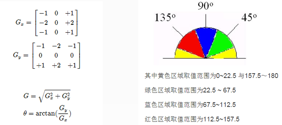 image
image
如图所示图片中的左侧是Sobel算子,$\theta$表示的是梯度的变化情况,看哪个方向上梯度变化更大,以此来确定角度。右图所示的就是角度区间。在每一个扇区,我们会对当前的像素和上下两个像素进行比较,如果当前的像素小于上下两个像素,那么上下两个像素保留,当前的像素舍弃,如果当前像素大于上下两个像素,那么上下两个像素被舍弃,当前像素保留。(我们只在每个扇区选择与他相近的两个像素)
高低阈值的选取
什么样的阈值是好的阈值,高低阈值到底该怎么选取呢?在实际编程中T1,T2为阈值,凡是高于T2的都保留,凡是小于T1都丢弃,从高于T2的像素出发,凡是大于T1而且相互连接的,都保留。最终得到一个输出二值图像。
推荐的高低阈值比值为 T2: T1 = 3:1/2:1 其中T2为高阈值,T1为低阈值。
cv::Canny
Canny(
InputArray src, // 8-bit的输入图像,不支持彩色图像,一定要提前转为灰度
OutputArray edges,// 输出边缘图像, 一般都是二值图像,背景是黑色
double threshold1,// 低阈值,常取高阈值的1/2或者1/3
double threshold2,// 高阈值
int aptertureSize,// Soble算子的size,通常3x3,取值3
bool L2gradient // 选择 true表示是L2来归一化,否则用L1归一化(L2是二范数,L1是一范数)
)
关于归一化,一般情况下为了计算速度,通常选择L1归一化。所以参数设置为false。
完整代码实现如下:
#include <opencv2/opencv.hpp>
#include <iostream>
#include <math.h>

using namespace cv;

Mat src, dst, gray_src;

int t1_value = 50;
int max_value = 255;

void Canny_Demo(int, void*);

int main(int argc, char** argv) {
	src = imread("D:/1.jpg");
	if (!src.data) {
		printf("could not load image...\n");
		return -1;
	}
	namedWindow("input image", CV_WINDOW_AUTOSIZE);
	namedWindow("output image", CV_WINDOW_AUTOSIZE);
	imshow("input image", src);

	cvtColor(src, gray_src, CV_BGR2GRAY);
	createTrackbar("Threshold Value:", "output image", &t1_value, max_value, Canny_Demo);  //创建一个拖动条,触发拖动条的回调函数为Canny_Demo
	Canny_Demo(0, 0);

	waitKey(0);
	return 0;
}

void Canny_Demo(int, void*) {
	Mat edge_output;
	blur(gray_src, gray_src, Size(3, 3), Point(-1, -1), BORDER_DEFAULT);
	Canny(gray_src, edge_output, t1_value, t1_value * 2, 3, false);

	/* 注释掉部分是用彩色图像显示canny算子,如果不加的话就是用黑白像素来显示canny算子处理结果,如果用彩色像素的话,处理速度会更慢一些
	dst.create(src.size(), src.type);
	src.copyTo(dst, edge_output);
	imshow("output image", dst);
	*/

	imshow("output image", edge_output);
}
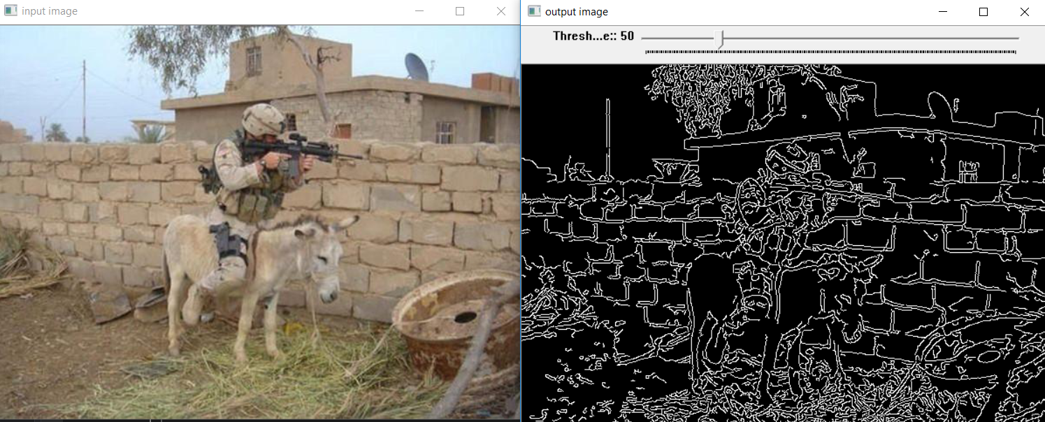
这样处理的图片最后是黑底,白色的边:
 image
image
如果翻转过来,改成白边黑底可能看起来效果会更好,我们只需要更改这个操作
imshow("output image", ~edge_output); //~表示取反,像素取反就可以变成白底黑边了
最后说一下,影响Canny算法的主要成像因素是低阈值和高阈值之间的选择。